Notes Part-2
Topics to be Learn : Part-2
|
Electric Field :
The region around a charged object in which coulomb force is experienced by another charge is called electric field.
Concept of electric field :
- Coulomb's law for the force exerted by one electric charge on another leads us to believe the interaction as direct and instantaneous charge ⇌
- The modern view introduces the concept of electric field to act as an intermediary between the charges. A charge sets up an electric field surrounding it, and the other charge interacts with the electric field of the first charge : charge ⇌ field ⇌
The concept of electric field is developed as follows.
- The presence of an isolated electric ‘source’ charge (or a certain collection of charges) in free space or any medium modifies the surrounding space such that another charge, called a test charge, placed in the vicinity experiences an electrostatic force \(\vec{F}\).
- \(\vec{F}\) is directly proportional to the magnitude of the test charge q0. However, the force per unit test charge, \(\vec{F}\)/q0, would be independent of the magnitude of the test charge. A test charge of a different magnitude would give exactly the same value of this quantity at the same point.
- The magnitude and direction of the force per unit test charge at various points represented as a map or a function completely describes the space surrounding the source charge(s).
- The quantity \(\vec{F}\)/q0 is called the electrostatic field \(\vec{E}\) of the source charge(s). The force on a charge q placed in the electric field \(\vec{E}\) is then \(\vec{F}\) = q\(\vec{E}\) .
Electric field intensity : The electric field intensity \(\vec{E}\) at a given point in space is defined as the electric force per unit charge exerted on a sufficiently small positive test charge placed at that point.
\(\vec{E}=\frac{\vec{F}}{q_0}\)
where is the force and q0 is the magnitude of the test charge.
SI unit and dimensions : The SI unit of electric field intensity is the newton per coulomb (N/C).
[E] = [F/ q0] = [MLT-2]/[TI] = [MLT-3I-1]
Electric Field Intensity due to a Point Charge in a Material Medium:
Consider a point charge q placed at point O in a medium of dielectric constant K (εr) as shown in Fig.

Consider the point P in the electric field of point charge q at distance r from it. A test charge q0 placed at the point P will experience a force which is given by the Coulomb’s law,
\(\vec{F}=\frac{1}{4πε_0K}.\frac{qq_0}{r^2}\hat{r}\)
where \(\hat{r}\) is the unit vector in the direction of force i.e., along OP.
By the definition of electric field intensity,
∴ \(\vec{E}=\frac{\vec{F}}{q_0}\) = \(\frac{1}{4πε_0K}.\frac{q}{r^2}\hat{r}\)
The direction of \(\vec{E}\) will be along OP when q is positive and along PO when q is negative.
Note :
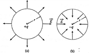
If we consider a sphere of radius r centred on a point source charge q, the magnitude (E) of the electric field intensity is the same at all points on the surface of the sphere. This is called spherical symmetry. At every point on the sphere, the electric field is radial — outward if q is positive and inward if q is negative]
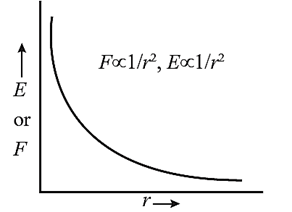
Graphical representation of variation of the magnitude of electric field intensity (or Coulomb force) due to a point charge with distance r from the charge :
The magnitude of electric field intensity in a medium is given by
E = \(\frac{1}{4πε_0K}.\frac{q}{r^2}\)
For air or vacuum K = 1 then
E = \(\frac{1}{4πε_0}.\frac{q}{r^2}\)
The coulomb force F between two charges and electric field E of a charge both follow the inverse square law,
Thus F ∝ 1/r2, E ∝ 1/r2
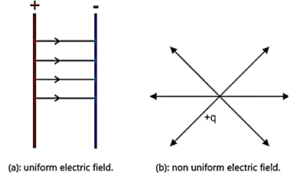
Uniform and non uniform electric field :
Uniform electric field: A uniform electric field is a field whose magnitude and
direction is same at all points.
- For example, field between two parallel plates. Fig (a)
Non uniform electric field: A field whose magnitude and direction is not the same at all points.
- For example, field due to a point charge. In this case, the magnitude of field is same at distance r from the point charge in any direction but the direction of the field is not same. Fig.(b)
Practical Way of Calculating Electric Field : Obtain relation E = V/d :
Consider a pair of identical metal plates held parallel to each other as shown in below Fig. The plates carry equal and opposite charges.
We assume that plates are very large and separated by a small distance d. Then the electric field in the region between the plates is uniform, except at the edges. We consider that region in which the field is uniform. If a charge + q is placed in this region, it is acted upon by the force \(\vec{F}\) = q\(\vec{E}\) due to the field (\vec{E}\), directed from the positive to the negative plate, i.e., in the direction of (\vec{E}\)
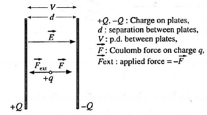
To move the charge from the negative to the positive plate without accelerating it, an external force equal to (-\vec{F}\) must be applied. The work done by the external force in this process is
W = Fd …..(1)
If V is the potential difference between the plates,
W = Vq ….(2)
From (1) and (2), we have, Vq = Fd
∴ \(\frac{V}{d}=\frac{F}{q}=\frac{qE}{q}\) = E
Thus, E = \(\frac{V}{d}\)
(This is the commonly used definition of electric field.)
Definition : The electric potential V at a point in an electric field is defined as the work per unit charge that must be done by an external agent against the electric force to move without acceleration a sufficiently small positive test charge from infinity to the point of interest.
V = W/q0 where W is the work done and q0 is the magnitude of the test charge. Electric potential is a scalar quantity.
Dimensions : [V] = [W]/[q0] = [ML2T—3I—1]
The dimensions of electric potential are 1 in mass, 2 in length, —3 in time and —1 in current.
SI unit: the volt (V) = the joule per coulomb (J/C).
Electric Lines of Force :
Consider an isolated, positive point charge q in vacuum. The electric field at every point in space around the charge is, by definition,
\(\vec{E}\) = \(\frac{1}{4πε_0}.\frac{q}{r^2}\hat{r}\)
According to the inverse-square law, the field is directed radially away from the positive charge and decreases in amplitude. These two field qualities can be represented by a series of straight lines going radially outward from the point charge, as shown in Fig. (a). The lines for a negative point charge point radially inward, as seen in Fig. (b). These lines are called the electric field lines or electric lines of force.
.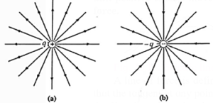
- The direction of a line is the direction of the electric field.
- The number of lines passing through a unit area that is perpendicular to the lines is proportional to the intensity of the electric field.
- Thus, the field lines are crowded together where the field is stronger; they are spread apart where the field is weaker.
- An electric field line also represents the path that would be followed by a test charge (initially at rest) when placed in the field.
Note : Michael Faraday (1791-1867) introduced the concept of lines of force for visualizing electric and magnetic fields. An electric line of force is an imaginary curve drawn in such a way that the tangent at any given point on this curve gives the direction of the electric field at that point.
Electric Field pattern : The lines of force are purely a geometric construction which help us visualise the nature of electric field in a region. The lines of force have no physical existence.
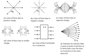
Characteristics of electric lines of force :
- The electric lines of force start from a positive charge and end on a negative charge.
- The tangent drawn to a line of force at any point gives the direction of the electric field intensity at that point.
- The lines of force do not intersect each other. If two lines of force intersect at a point, it would mean electric field has two directions at that point. This is impossible.
- The lines of force do not pass through a conductor, but they can pass through a dielectric, i.e., nonconducting medium.
- The lines of force are crowded in a region where the intensity of electric field is large. They are widely separated in a region where the intensity is small.
- The number of lines of force per unit area of the surface held perpendicular to the electric field is proportional to the magnitude of the electric field intensity there.
- In a nonuniform electric field, the lines of force are curved. In a uniform electric field, lines of force are straight lines, parallel to each other and equidistant.
- The lines of force are always perpendicular to the surface of a conductor carrying static charges.
Electric Flux :
The total number of electric lines of force passing normally through a given area in an electric field, is called the electric flux through that area.
∴ E = (Number of lines of force)/(Area enclosing the lines of force)
∴ Number of lines of force = (E).(Area)
When the area is inclined at an angle θ with the direction of electric field, Fig., the electric flux can be calculated as follows.
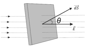
Consider a very small area dS in an electric field of intensity \(\vec{E}\). The area dS is assumed to be so small that the electric field intensity at every point of this area can be considered to be the same as \(\vec{E}\).
The area dS can be represented by a vector \(\vec{dS}\) drawn perpendicular to it. Let θ be the angle between \(\vec{E}\) and \(\vec{dS}\).
Then the electric flux through the area dS is
dΦ = E dS cos θ = \(\vec{E}.\vec{dS}\) because E cos θ is the component of \(\vec{E}\) along \(\vec{dS}\).
Thus, the electric flux through a small area drawn in an electric field is equal to the scalar product of the intensity (\(\vec{E}\)) and the area vector (\(\vec{dS}\)).
When the surface is large, the electric flux through it is
Φ = ∫ \(\vec{E}.\vec{dS}\) = ∫ E dS cos θ
The SI unit of electric intensity is N/C or V/m and that of area is m2. Hence, from the above relation, the SI unit of electric flux is N-m2/C which is the same as the volt-metre (V.m).
(i) For θ = 0, cos θ = 1 ∴ dΦ = E dS
(ii) For θ = 90°, cos θ = 0 ∴ dΦ = 0
(ii) For θ = 45°, cos θ = \(\frac{1}{\sqrt{2}}\), ∴ dΦ = \(\frac{1}{\sqrt{2}}\)E dS
Gauss' Law :
Gauss’s theorem : The flux of the net electric field through a closed surface equals the net charge enclosed by the surface divided by ε0 (in free space).
Proof : Consider a closed surface of arbitrary shape surrounding a positive point charge Q at a point O in free space, see below Fig.
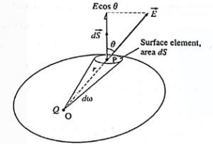
Consider a small element of the surface, of area dS around a point P at a distance r from point O. Area dS is assumed to be so small that every point on it can be considered to be at the same distance r from O and the electric field over it can be considered to be uniform.
The magnitude of the electric field intensity at P is
E = \(\frac{Q}{4πε_0r^2}\) ….(1)
where ε0 is the absolute permittivity of free space. The outward normal drawn to the area element makes an angle θ with the electric field. Hence, the electric flux through area dS is
dΦ = E dS cos θ.
= \((\frac{Q}{4πε_0r^2})\)dS cos θ
= \(\frac{Q}{4πε_0}.\frac{dS\,cos\,θ}{r^2}\) …..(2)
\(\frac{dS\,cos\,θ}{r^2}\) is the solid angle dw subtended by the area dS at point O.
∴ dS = \(\frac{Q}{4πε_0}\)dω ….(3)
The electric flux through the closed surface = \(\oint \frac{Q}{4πε_0}dω\) = \(\frac{Q}{4πε_0}\oint dω\) ….(4)
A closed surface subtends a solid angle of 4π steradians at any point inside it, i.e., \(\oint dω\) = 4 π steradians.
∴ The electric flux through the closed surface = \(\frac{Q}{4πε_0} x 4π = Q/ε0 ….(5)
Instead of a single free charge, if there are many free charges Q1, Q2, Q3, etc., we can write Eq. (4) for each point charge and then sum over all the charges.
∴ The electric flux through the closed surface = ∑Q/ ε0.
where ∑Q = Q1 + Q2 + Q3 +... is the algebraic sum of all free charges, i.e., the net charge enclosed by the surface. This is Gauss's law in mathematical form.
Electric Dipole :
A pair of equal and opposite charges separated by a finite distance is called an electric dipole.
Below figure shows an electric dipole consisting of two point charges + q and — q separated by a small distance 2l, called the dipole length.

- The line joining the two charges is called the dipole axis.
- The point O, midway between the charges, is the centre of the dipole.
- A line through O and perpendicular to the dipole axis is called dipole equator.
- Though the total charge of the dipole is zero, the dipole produces electric field.
- All distances from the dipole are measured from its centre O.
Definition : The electric dipole moment of a given dipole is a vector whose magnitude is the product of the magnitude of the charge and the distance between the two charges, and is directed from the negative to the positive charge of the dipole.
If the magnitude of the charge at each pole of an electric dipole is q and the dipole length is 2l, the electric dipole moment of the dipole is
\(\vec{p}\) = q(2\(\vec{l}\))
where 2\(\vec{l}\) is directed from the negative to the positive charge.
Dimensions : [p] = [q] [2 l] = [TI] [L] = [LTI]
Unit ; The SI unit of electric dipole moment is the coulomb-metre (C.m). The debye (D) is a non SI unit of electric dipole moment.
1 debye = 3.33564 x 10—30 coulomb-metre.
Couple Acting on an Electric Dipole in a Uniform Electric Field:
Expression :
Consider an electric dipole consisting of a pair of opposite charges, each of magnitude q and dipole length 2 l. Suppose it is placed in a uniform electric field \(\vec{E}\) with its axis inclined at an angle θ to \(\vec{E}\) as shown in Fig.

The electrostatic force on the positive charge is q\(\vec{E}\), and that on the negative charge is — q\(\vec{E}\). That is, these forces both have magnitude qE, act in opposite directions and, in general, have different lines of action. They are shown in the figure as \(\vec{F}\) and \(-\vec{F}\) . These two equal and opposite forces constitute a couple which tends to line up the electric dipole moment with the field \(\vec{E}\).
The torque of the couple (in the clockwise sense in above Fig.), in magnitude, is the product of the magnitude of any of the forces constituting the couple and the perpendicular distance between their lines of action.
τ = Fd = (qE) (2l sin θ) = pE sin θ
where p = q (2 l ) is the magnitude of the electric dipole moment and θ is the smaller of the two angles between \(\vec{p}\) and \(\vec{E}\). Expressing the torque as a vector product,
\(\vec{τ}\) = \(\vec{p}\) x \(\vec{E}\)
This is the expression for the torque on an electric dipole of moment \(\vec{p}\) in a uniform electric field of intensity \(\vec{E}\).
Note : τ = 0 for θ = 0° and 180°. τ = τmax =pE for θ = 90°
Electric Intensity at a Point due to an Electric Dipole:
Consider an electric dipole with charges +q and —q separated by a small distance 2l.
Let the dipole axis be the x—axis with the unit vector \(\hat{i}\) directed from —q to + q. The origin is taken at the centre of the dipole. The electric dipole moment
\(\vec{p}\) = \(q(2\vec{l})\) = \(q(2l)\hat{i}\)
Case 1 : At a point on the axis of a dipole.

The electric field intensity \(\vec{E}_{axis}\) on the dipole axis at point A (see below Fig.) has a term \(\vec{E}_1\) from charge + q and a term \(\vec{E}_2\) from charge —q.
\(\vec{E}_1\) = \(\frac{1}{4πε_0}.\frac{q}{(x-l)^2}\hat{i}\)
and
\(\vec{E}_2\) = \(\frac{1}{4πε_0}.\frac{-q}{(x+l)^2}\hat{i}\)
∴ \(\vec{E}_{axis}\) = \(\vec{E}_1\)+\(\vec{E}_2\)
= \(\frac{1}{4πε_0}q[\frac{1}{(x-l)^2}-\frac{1}{(x+l)^2}]\hat{i}\)
= \(\frac{1}{4πε_0}q[\frac{(x+l)^2-(x-l)^2}{((x-l)(x+l))^2}]\hat{i}\)
= \(\frac{1}{4πε_0}\frac{q(4xl)}{(x^2-l^2)^2}\hat{i}\)
= \(\frac{1}{4πε_0}\frac{2\vec{p}x}{(x^2-l^2)^2}\) (‘.’ \(\vec{p} = q2l\hat{i}\))
For a far-field approximation or for a short dipole (x >> l), l2 << x2 and the term l2 can be omitted from the denominator.
Then
\(\vec{E}_{axis}\) ≈ \(\frac{1}{4πε_0}\frac{2\vec{p}x}{x^4}\) = \(\frac{1}{4πε_0}\frac{2\vec{p}}{x^3}\)
\(\vec{E}_{axis}\) has the same direction as that of \(\vec{p}\)
Case 2: At a point on the equatorial line.
Equatorial field : A point B on the equator of the dipole is equidistant from both the charges. So the field \(\vec{E}_1\) due to charge + q and \(\vec{E}_2\) due to charge — q are equal in magnitude. \(\vec{E}_1\) is directed away from + q while \(\vec{E}_2\) is directed towards — q, see below Fig.

Resolving \(\vec{E}_1\) and \(\vec{E}_2\) along the x- and y-axis, we see that the equal and opposite y-components E1y and E2y cancel out. The resultant field at B is, thus, due to the sum of the x—components, E1x and E2x which too are equal in magnitude.
Eequator = E1x + E2x = 2E1x = 2 E1 cos θ
From the figure, the distance of the point B from the charge + q is \(\sqrt{y^2+l^2}\), so that
cos θ = \(\frac{l}{\sqrt{y^2+l^2}}\)
and E1 = \(\frac{1}{4πε_0}.\frac{q}{y^2+l^2}\)
∴ Eequator = 2\([\frac{1}{4πε_0}.\frac{q}{y^2+l^2}.\frac{l}{\sqrt{y^2+l^2}}]\)
= \(\frac{1}{4πε_0}.\frac{p}{(y^2+l^2)^{3/2}}\)
Since this resultant field is opposite to the dipole moment,
\(\vec{E}_{equator}\) = \(\frac{1}{4πε_0}.\frac{-\vec{p}}{(y^2+l^2)^{3/2}}\)
For a far-field approximation or for a short dipole (y>> 1),
∴ \(\vec{E}_{equator}\) = \(\frac{1}{4πε_0}.\frac{-\vec{p}}{y^3}\)
- At the same distance from the dipole centre, x = y, Eaxis = 2Eequator, for a short dipole.
- The field intensities Eaxis and Eequator, far from the dipole, are both proportional to the dipole moment and inversely proportional to the cube of the distance from the dipole centre.
Continuous Charge Distribution :
- The excess electric charge on a charged body is always an integral multiple of the electronic (or elementary) charge e, and hence discrete.
- On the macroscopic scale, however, the charge on a body is so large compared to the electronic charge that the discreteness is not noticeable.
- It seems that the charge on the body can change by continuous amounts. Then the body is said to have continuous distribution of charge.
- A continuous distribution of charge can be uniform or nonuniform. Charges can move freely on a conductor.

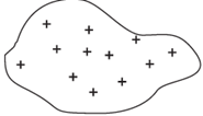
- When a charged conducting sphere is far from external charges, it has a uniform distribution of charges on its outer surface, Fig. (a).
- When an external charge is brought near the charged conducting sphere, the charge distribution on the sphere becomes nonuniform, Fig. (b).
- Also, when a conductor is not spherical, the charge distribution is nonuniform, Fig.
To find the electric field due to continuous charge distribution, we define following terms for different types of charge distribution :
(i) Linear charge density (λ) : The electric charge per unit length of a one dimensional body (such as a wire, whose diameter is negligible compared to its length) is called linear charge density λ.
λ = q/l
Example: Charge distributed uniformly on a straight thin rod or a thin nylon thread.
![]()
If the charge is not distributed uniformly over the length of thin conductor then charge dq on small element of length dl can be written as dq = λdl
Dimensions : [L—1TI], SI unit of λ is (C/m).
(ii) Surface charge density (σ ) : The electric charge per unit area of a surface is called the surface charge density σ.
σ = q/A
Example : Charge distributed uniformly on a thin disc or a synthetic cloth.
If the charge is not distributed uniformly over the surface of a conductor, then charge dq on small area element dA can be written as dq = σ dA.
Dimensions : [L—2TI], SI unit of σ is (C/m2).
(iii) Volume charge density (ρ) : The electric charge per unit volume of a medium or body is called its volume charge density ρ.
ρ = q/V
Example : Charge on a solid plastic sphere or a solid plastic cube.
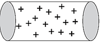
If the charge is not distributed uniformly over the volume of a material, then charge dq over small volume element dV can be written as dq = ρ dV.
Dimensions : [L—3TI], SI unit of ρ is (C/m3).
Know This :
Static charge can be useful
- Static charges can be created whenever there is a friction between an insulator and other object.
- Example : When an insulator like rubber or ebonite is rubbed against a cloth, the friction between them causes electrons to be transferred from one to the other. This property of insulators is used in many applications such as Photocopier, Inkjet printer, Panting metal panels, Electrostatic precipitation/separators etc.
Static charge can be harmful
- When charge transferred from one body to other is very large sparking can take place. For example lightning in sky.
- Sparking can be dangerous while refueling your vehicle.
- One can get static shock if charge transferred is large.
- Dust or dirt particles gathered on computer or TV screens can catch static charges and can be troublesome.
Precautions against static charge
- Home appliances should be grounded.
- Avoid using rubber soled footwear.
- Keep your surroundings humid. (dry air can retain static charges).
We reply to valid query.