Notes
|
Topics to be learn :
|
Introduction of Statistics :
- Statistics is the field of mathematics that collects, presents, analyzes, and interprets numerical data.
- Statistics are utilized in all aspects of life. It has applications in agriculture, botany, biotechnology, bioinformatics, chemistry, physics, economics, commerce, geography, sociology, and medicine, among other fields.
- An experiment can have several outcomes. The record can be used to examine the possibilities for various outcomes. Statistical criteria are used to do this.
Measures of a central tendency :
We usually find a specific property in the numerical data collected in a survey that the scores have a tendency to cluster around a particular score. This score is a representative of the group. The number is called the measure of the central
tendency.
We have studied the measure of the central tendency, namely the mean, median and mode for ungrouped data.
The mean of statistical data = \(\frac{\text{The sum of all scores}}{\text{Total no. of scores}}=\frac{∑_{i=1}^{N}x_i}{N}\)
(Here, xi is the i th score)
The mean is denoted by \(\bar{X}\). It represents the average of the given data
\(\bar{X} = \frac{∑_{i=1}^{N}x_i}{N}\)
Mean from classified frequency distribution :
When the number of scores in a data is large, we use some different methods to find the sum. The methods are :
- Direct method
- Assumed mean method
- Step deviation method
(i) Direct method :
Ex. (1) The percentage of marks of 50 students in a test is given in the following table. Find the mean of the percentage
| Percentage of marks | 0-20 | 20-40 | 40-60 | 60-80 | 80-100 |
| No. of students | 3 | 7 | 15 | 20 | 5 |
Solution :
(1) Vertical columns are drawn as shown in the table.
(2) Classes are written in the first column.
(3) The class mark xi is in the second column.
(4) In the third column, the number of workers, that is frequency (fi) is written.
(5) In the fourth column, the product (xi × fi) for each class is written.
(6) Then ∑ xi fi is written.
| Class (Percentage of
marks) |
Class mark
xi |
Frequency
(No. of students) fi |
Class mark frequency
xi fi |
| 0-20 | 10 | 3 | 30 |
| 20-40 | 30 | 7 | 210 |
| 40-60 | 50 | 15 | 750 |
| 60-80 | 70 | 20 | 1400 |
| 80-100 | 90 | 5 | 450 |
| Total | N=∑ fi = 50 | ∑ xi fi = 2840 |
(7) The mean is found using the formula
Mean = \(\bar{X} = \frac{∑x_if_i}{N}=\frac{2840}{50}\) = 56.8
∴ The mean of the percentage = 56.8
(ii) Assumed mean method :
In the examples solved above, we see that some times the product xi fi is large. If the product xi fi is large, it becomes difficult to calculate the mean by direct method. Finding the mean by 'assumed mean method' becomes simpler if we use addition and division in this method.
Ex. : The daily sale of 100 vegetable vendors is given in the following table. Find the mean of the sale by assumed mean method.
| Daily sale (Rupees) | 1000-1500 | 1500-2000 | 2000-2500 | 2500-3000 |
| No. of vendors | 15 | 20 | 35 | 30 |
Steps to calculate mean by this method :
(1) Assumed mean, A. In this example A = 2250. (Generally, the class mark of the
class having maximum frequency is chosen as the assumed mean.)
(2) In column 1, write the class intervals. (Here daily sale)
(3) Class marks are written in the second column.
(4) Values of di = xi — A, write in the third column.
(5) In column 4, write the frequencies (fi). Write ∑ fi at the bottom of this column.
(6) In the fifth column, the product (fi × di) and their sum is written as ∑ fi di.
\(\bar{d}\) and \(\bar{X}\) are calculated using the formulae.
\(\bar{d} = \frac{∑f_id_i}{f_i}\), Mean \(\bar{X}\) = A + \(\bar{d}\)
| Class daily sale (Rupees) | Class mark
xi |
di = xi- A = xi- 2250 | Frequency (No. of vendors)
fi |
Frequency × Deviation
fi × di |
| 1000-1500 | 1250 | -1000 | 15 | -15000 |
| 1500-2000 | 1750 | -500 | 20 | -10000 |
| 2000-2500 | 2250→A | 0 | 35 | 0 |
| 2500-3000 | 2750 | 500 | 30 | 15000 |
| Total | N=∑ fi = 100 | ∑ fi di = -10000 |
Assumed mean = A = 2250, di = xi - A is the deviation
\(\bar{d} = \frac{∑f_id_i}{f_i}=\frac{10000}{100}\) = —100
∴ Mean = A + \(\bar{d}\) = 2250 — 100 =2150
The mean of sale is Rs. 2150.
(iii) Step Deviation Method :
This method reduces the calculations still further.
Steps to calculate mean by this method :
(1) In column 1, write the given class interval. (Amount invested in below example).
(2) In column 2, write the corresponding class marks (xi).
(3) In column 3, write the values of di where di = xi — A.
(4) Find g, the GCD of all di. In column 4, write the values of ui, where
ui = \(\frac{x_i-A}{g}=\frac{di}{g}\)
(5) In column 5, write the frequencies (fi) of the given class intervals. Find their sum (∑fi).
(6) In column 6, write fi ui . Find their sum ( ∑fiui).
Find using the formula, \(\bar{u}=\frac{∑f_iu_i}{f_i}\)
Find mean, \(\bar{X}\) = A + g\(\bar{u}\)
Example : The amount invested in health insurance by 100 families is given in the following frequency table. Find the mean of investments using step deviation method.
| Amount invested (Rupees) | 800-1200 | 1200-1600 | 1600-2000 | 2000-2400 | 2400-2800 | 2800-3200 |
| No. of families | 3 | 15 | 20 | 25 | 30 | 7 |
Solution :
Assumed mean A = 2200 observing all ‘di’ s g = 400. (g=greatest common divisor)
| Class (Insurance Rs.) | Class mark
xi |
di = xi- A = xi- 2200 | ui = \(\frac{di}{g}\) | Frequency (No. of families)
fi |
fi × ui |
| 800-1200 | 1000 | -1200 | -3 | 3 | -9 |
| 1200-1600 | 1400 | -800 | -2 | 15 | -30 |
| 1600-2000 | 1800 | -400 | -1 | 20 | -20 |
| 2000-2400 | 2200 | 0 | 0 | 25 | 0 |
| 2400-2800 | 2600 | 400 | 1 | 30 | 30 |
| 2800-3200 | 3000 | 800 | 2 | 7 | 14 |
| Total | N = ∑fi = 100 | ∑ fi ui = -15 |
Here ∑ fi ui = -15, ∑fi = 100, g = 400
\(\bar{u}=\frac{∑f_iu_i}{f_i} =\frac{-15}{100}\) = -0.15
Mean, \(\bar{X}\) = A + g\(\bar{u}\) = 2200 + (-0.15) × 400 = 2200 – 60 = 2140
∴ The mean of investments in health insurance = Rs. 2140.
Median for grouped frequency distribution :
Formula for finding the median of a grouped frequency distribution :
Median = L + \([\frac{\frac{N}{2}-cf}{f}]\) × h
where, L = lower class limit of the median class.
N =sum of frequencies
cf = cumulative frequency of the class preceding the median class.
f =frequency of the median class.
h =class interval of the median class.
Following are the steps in the calculation of median for grouped frequency distribution:
- Prepare a table containing three columns
- Write the given class intervals in column 1 and their respective frequencies in column 2.
- Write cumulative frequency less than type in column 3.
- Find total frequency N = ∑fi. Calculate \(\frac{N}{2}\)
- Find cumulative frequency less than type which is just greater than or equal to g.
- The corresponding class is median class.
- Calculate the value of the median by using the formula given above.
[Note : If the class intervals are of inclusive type, make them exclusive type by finding class boundaries. ]
Example :
The following table shows frequency distribution of marks of 100 students of 10th class which they obtained in a practice examination. Find the median of the marks.
| Marks in exam | 0-20 | 20-40 | 40-60 | 60-80 | 80-100 |
| No. of students | 4 | 20 | 30 | 40 | 6 |
Solution :
| Class (Student’s marks ) | No. of students
fi |
Cumulative frequency less than the upper limit
cf |
| 0-20 | 4 | 4 |
| 20-40 | 20 | 20+4=24 |
| 40-60 (median class) | 30 | 30+24=54 |
| 60-80 | 40 | 40+54=94 |
| 80-100 | 6 | 6+94=100 |
Here, total of frequencies N = ∑fi = 100
\(\frac{N}{2}=\frac{100}{2}\) = 50. Cumulative frequency which is just greater than 50 is 54.
∴ the corresponding class 40-60 is the median class.
L = 40, f = 30 (Frequency of the median class), cf = 24, h = 20
Median = L + \([\frac{\frac{N}{2}-cf}{f}]\)× h
= 40 + \([\frac{\frac{100}{2}-24}{30}]\)× 20 = 40 + \(\frac{50-24}{30}\)× 20
= 40 + \(\frac{26}{30}\)× 20 = 40 + 17\(\frac{1}{3}\)
= 57\(\frac{1}{3}\)
∴ median of the marks = 57\(\frac{1}{3}\)
Remember :
- If the given classes are not continuous, we have to make them continuous to find out the median.
- It is difficult to write the scores in the asscending order when the number of scores is large. So the data is classified into groups. It is not possible to find the exact median of a classified data, but the approximate median is found by the formula.
Median = L + \([\frac{\frac{N}{2}-cf}{f}]\)× h
Mode for grouped frequency distribution :
Mode : The score repeating maximum number of times in a data is called the mode of the data.
The following formula is used to estimate the mode of grouped data.
Mode = L + \([\frac{f_1-f_0}{2f_1-f_0-f_2}]\)× h
In the above formula,
L = Lower class limit of the modal class.
f1 = Frequency of the modal class.
f0 =Frequency of the class preceding the modal class.
f2 = Frequency of the class succeeding the modal class.
h = Class interval of the modal class.
Example : The classification of children according to their ages, playing on a ground is shown in the following table. Find the mode of ages of the children.
| Age-group of children (Yrs) | 6-8 | 8-10 | 10-12 | 12-14 | 14-16 |
| No. of children | 43 | 58 | 70 | 42 | 27 |
Solution :
Here the maximum number of children is of the age - group 10-12. So the modal class is 10-12.
∴ in the given example,
L = Lower class limit of the modal class = 10
h = Class interval of the modal class = 2
f1 = Frequency of the modal class = 70
f0 = Frequency of the class preceding the modal class = 58
f2 = Frequency of the class succeeding the modal class = 42
Mode = L + \([\frac{f_1-f_0}{2f_1-f_0-f_2}]\)× h
= 10 + \([\frac{70-58}{2(70)-58-42}]\)× 2
= 10 + \(\frac{12}{40}\)× 2
= 10 + \(\frac{24}{40}\)
= 10 + 0.6 = 10.6
∴ the mode of the ages of children playing on the ground is 10.6 Years.
Remember :
- We have studied the central tendencies mean, median and mode. Before selecting any of these measures, we have to know the purpose of its selection clearly.
- Suppose, we have to judge the performance of five divisions of standard 10 in the internal examination. For the purpose, we have to find the 'mean' of marks of students in each division.
- If we have to make two groups of students in a division based on their marks in the examination, we have to find the 'median' of their marks.
- If a 'bachat' group producing chalks wants to know about the colour of chalks having maximum demand, it will have to choose the 'mode'.
Pictorial representation of statistical data :
The mean, median or mode of a numerical data or analysis of the data is useful to draw some useful inferences. The tabulation is one of the methods representing numerical data in brief. A table does not immediately convey some characteristics of the data. A common man is interested in the important aspects of a data.
Presentation of data :
Pictorial and graphical presentation are attractive methods of data interpretation.
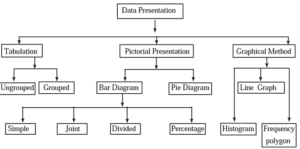
The tree chart below shows different methods of data interpretation.
We have studied some of these methods and graphs in previous standards. Now we will learn a histogram, a frequency polygon and a pie diagram.
(i) Histogram :
Method of drawing a histogram :
- If the given classes are not continuous, make them continuous. Such classes are called extended class intervals.
- Show the classes on the X-axis with a proper scale.
- Show the frequencies on the Y-axis with a proper scale.
- Taking each class as the base, draw rectangles with heights proportional to the frequencies.
- On the X-axis, a mark ‘
 ‘ called the krink mark is shown between the origin and the first class.
 - It means, there are no observations up to the first class. The mark can be used on the Y-axis also, if needed. This enables us to draw a graph of optimum size.
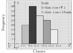
Example : The table below shows the net asset value (NAV) per unit of mutual funds of some companies. Draw a histogram representing the information.
| NAV (Rs.) | 8-9 | 10-11 | 12-13 | 14-15 | 16-17 |
| No. of mutual funds | 20 | 40 | 30 | 25 | 15 |
Solution :
The given classes are not continuous. Lets make the classes continuous.
Continuous Classes |
7.5-9.5 | 9.5-11.5 | 11.5-13.5 | 13.5-15.5 | 15.5-17.5 |
| Frequency | 20 | 40 | 30 | 25 | 15 |
(ii) Frequency polygon :
A frequency polygon is another way of presentation. Two methods of drawing a frequency polygon is: (a) With the help of a histogram (b) Without the help of a histogram.
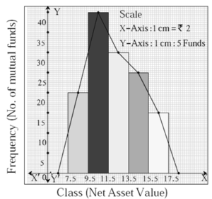
(a) With the help of a histogram :
Steps :
- Draw a histogram from the given information.
- Mark the midpoint of the upper side of each rectangle of the histogram.
- Take one additional rectangle of height zero preceding the first rectangle and one more additional rectangle of height zero succeeding the last rectangle. Mark the midpoints of these two rectangles. Such marks will be on the X-axis.
- Join the successive midpoints by line segments and get a closed figure. It is a frequency polygon.
Example : Here, we have used the histogram figure of above example to learn the method of drawing a frequency polygon.
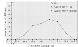
(b) Without the help of a histogram :
Decide the coordinates of each point with respect to each class. Plot the points on a graph paper. Join successive points by a straight line and get a frequency polygon.
Example : The following table shows the weights of children and the number of children. Draw a frequency polygon showing the information.
| Weight of children (kg) | 18-19 | 19-20 | 20-21 | 21-22 | 22-23 | 23-24 |
| No. of children | 4 | 13 | 15 | 19 | 17 | 6 |
Solution :
Let us prepare a table showing the co-ordinates necessary to draw a frequency polygon.
| Class | 18-19 | 19-20 | 20-21 | 21-22 | 22-23 | 23-24 |
| Class mark | 18.5 | 19.5 | 20.5 | 21.5 | 22.5 | 23.5 |
| Frequency | 4 | 13 | 15 | 19 | 17 | 6 |
| Coordinates of points | (18.5, 4) | (19.5,13) | (20.5,15) | (21.5,19) | (22.5,17) | (23.5,6) |
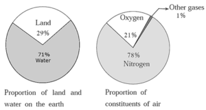
(iii) Pie diagram :
In a pie diagram, the numerical data is shown in a circle. Different components of the data are shown by proportional sectors of the circle.
Reading of Pie diagram :
The following example illustrates how a pie chart gives information at a glance.
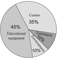
Figure shows the annual financial planning of a school. From the pie diagram we see that
- 45% of the amount is reserved for educational equipment.
- 35% of the amount is shown for games.
- 10% of the amount is kept for sanitation.
- 10% of the amount is reserved for environment.
To draw a Pie diagram :
- To draw a pie diagram, the whole circle is divided into sectors proportional to the components of the data.
- The measure of central angle of each sector is found by the following formula.
- The measure of central angle of sector θ = \(\frac{\text{Number of scores in component}}{\text{Total number of scores}}\)x 360°
- A circle of a suitable radius is drawn. Then it is divided into sectors such that, the number of sectors is equal to the number of components in the data.
Example :
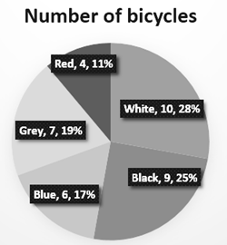
(i) In a bicycle shop, number of bicycles purchased and choice of their colours was as follows. Find the measures of sectors of a circle to show the information by a pie diagram.
Solution :
In all 36 bicycles were purchased. Out of them 10 bicycles were white coloured.
∴ Measure of sector showing white coloured bicycles = \(\frac{\text{Number of white bicycles}}{\text{Total number of bicycles}}\) x 360
= \(\frac{10}{36}\)x 360 = 100
The measures of angles of sector relating to bicycles of other colours can be calculated similarly which are shown in the adjacent table.
| Colour | Number of bicycles | Central angle of the sector |
| White
Black Blue Grey Red |
10
9 6 7 4 |
100°
90° 60° 70° 40° |
| Total | 36 | 360° |
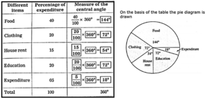
(ii) The monthly expenditure of a family on different items is shown in the following table. Calculate the related central angles and draw a pie chart.

Solution :
We reply to valid query.