Notes
|
Topics to be Learn : Part-1
|
Introduction :
Facts about magnetism :
- The north and south poles are the two poles that are present in every magnet, regardless of size or shape.
- If a magnet is broken into two or more pieces then each piece behaves like an independent magnet with somewhat weaker magnetic field. Thus isolated magnetic monopoles do not exist.
- Like magnetic poles repel each other, whereas unlike poles attract each other.
- When a bar magnet/ magnetic needle is suspended freely or is pivoted, it aligns itself in geographically North-South direction.
Magnetic Lines of Force and Magnetic Field :
Magnetic flux (Φ) : The number of magnetic field lines passing through a surface, held perpendicular to the lines, is called the magnetic flux through the surface.
SI unit : the weber, 1 Wb = 1 N.m/A, named in honour of Wilhelm E. Weber (1804 — 91) German physicist.
(Note : Magnetic field lines were earlier called as magnetic lines of force.)
Magnetic induction : The magnitude of the magnetic induction at a point in a magnetic field is defined as the magnetic flux density (the magnetic flux per unit area) across an infinitesimal surface, containing the point, at right angles to the magnetic field lines.
Magnetic Field (B) = magnetic flux(Φ)/area(A)
SI unit : the tesla, 1 T = 1 Wb/m2. 1 tesla = 104 gauss (G).
The quantity \(vec{B}\) properly called as magnetic field induction. The magnetic field ‘strength’ or intensity, denoted by \(vec{H}\) is different from \(vec{B}\)
SI unit of magnetic intensity H : The ampere per metre (A/m).
CGS unit of H : oersted (Oe), 1 Oe = 79.6 A/m.
Properties of magnetic field lines or lines of force :
Magnetic lines of force originate from the north pole and end at the south pole of a bar magnet. The magnetic lines of force of a magnet have the following properties:
- Closed loops are formed by the magnetic lines of force of a magnet or a solenoid. In the case of an electric dipole, the electric lines of force begin at the positive charge and terminate on the negative charge without making a full loop.
- The direction of the net magnetic field \(vec{B}\) at a point is given by the tangent to the magnetic line of force at that point in the direction of line of force.
- The number of lines of force crossing per unit area decides the magnitude of the magnetic field \(vec{B}\).
- The magnetic lines of force do not intersect. This is because had they intersected, the direction of magnetic field would not be unique at that point.
The Bar magnet :
Concept of magnetic poles :
- Quantitative measurements show that in many respects the force between the poles of two magnets is similar to the Coulomb force between electric charges.
- In particular, they exhibit the same inverse square dependence on distance.
- Hence, analogous to an electric dipole, we hypothesize that there are positive (N) and negative (S) magnetic charges within a magnet.
- Also, they are assumed to act as the source of the magnetic field in exactly the same way that electric charges act as the source of electric field.
Therefore, assuming that magnetic charges as such exist, we view a bar magnet as a magnetic dipole : two magnetic charges of opposite polarity at its two poles (N and S), a distance 2l apart. The magnitude of each ‘magnetic charge’ is referred to as its ’pole strength’ and is equal to qm = \(\frac{m}{2l}\), where is the magnetic dipole moment, pointing from the negative (or south, S) pole to the positive (or north, N) pole.
- SI unit of pole strength (qm) is A.m.
- SI unit of magnetic dipole moment m is A.m2.
Magnetic dipole : The most elementary magnetic structure behaves as a pair of two magnetic poles of opposite types (north and south or positive and negative) and of equal strengths; isolated magnetic poles are not observed. Thus, a magnetic dipole is a pair of two magnetic poles of opposite types and equal strengths a finite distance apart.
A bar magnet is an example of a magnetic dipole. Since the magnetic field lines are closed loops, the positions of the poles cannot be accurately determined. In the case of a bar magnet, the positions of the poles are conjectured to be the points inside the magnet where the field lines appear to meet when extrapolated.

Magnetic length : In a magnetic dipole, the finite distance between the two poles is called its magnetic length. For the sake of convenience, it is denoted by 2l, so that the distance of each pole from the centre of the dipole is l. In the case of a bar magnet, an approximate relation exists between the magnetic length and the geometric length :
magnetic length, 2l = \(\frac{5}{6}\)(geometric length, L)
Magnetic axis : The line through the two poles of a magnetic dipole is called the magnetic axis of the dipole.
Magnetic equator : A line through the centre of a magnetic dipole and perpendicular to its magnetic axis is called a magnetic equator of the dipole. (An equatorial plane is perpendicular to the magnetic axis and contains the magnetic equator.)
Magnetic field due to a bar magnet at a point along its axis and at a point along its equator:
Consider a bar magnet of magnetic dipole moment \(vec{m}\) and magnetic length 2l.
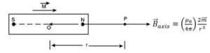
(i) Along its axis : Consider a point P on the axis of the magnet at a distance r from the centre of the magnet. The magnetic induction at P, called the axial
magnetic field, is
\(\vec{B}_{axis}=(\frac{μ_0}{4π})\frac{2\vec{m}r}{(r^2-l^2)^2}\)
where μ0 is the permeability constant for vacuum. \(\vec{B}_{axis}\) and \(vec{m}\) have the same direction.
If the magnet is very short, i.e., l << r, we can ignore l2: in the denominator in comparison with r2.
∴ \(\vec{B}_{axis}=(\frac{μ_0}{4π})\frac{2\vec{m}}{r^3}\)
Thus, for a short magnet the induction varies inversely as the cube of the distance from it.
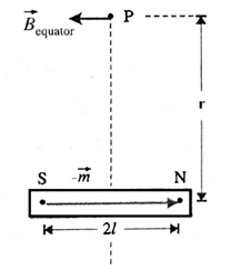
(ii) Along its equator: Consider a point P on the equator of the magnet at a distance r from the centre of the magnet.
The magnetic induction at P, called the equatorial magnetic field, is
\(\vec{B}_{eq}=(\frac{μ_0}{4π})\frac{-\vec{m}}{(r^2+l^2)^{3/2}}\)
The minus sign shows that the direction of \(\vec{B}_{eq}\), is opposite to that of \(vec{m}\).
If the magnet is very short, i.e., l << r, we can we can ignore l2: in the denominator in comparison with r2. We the get,
\(\vec{B}_{eq}=(\frac{μ_0}{4π})\frac{(-\vec{m})}{r^3}\)
Thus, for a short magnet the induction varies inversely as the cube of the distance from it.
Magnetic field due to a bar magnet at an arbitrary point:
Consider a short magnetic dipole of magnetic length 2l and magnetic dipole moment \(vec{m}\) directed from the south pole to the north pole.
We wish to find the magnetic induction at a point P, at a distance r from the centre O of the dipole; OP makes an angle θ with the dipole axis, as shown in Fig.
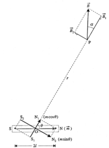
Resolve the magnetic moment \(vec{m}\) into two components, along OP and perpendicular to OP. Then, the given dipole SN can be considered as a combination of two dipoles : S1N1 with magnetic moment m cos θ (in magnitude) and S2N2 with magnetic moment m sin θ (in magnitude).
Let \(vec{B}_1\) and \(vec{B}_2\) be the magnetic inductions at P due to S1N1 and S2N2 respectively.
Point P lies on the axis of the dipole S1N1.
∴ B1 = \(\frac{μ_0}{4π}\frac{2m\,cos\,θ}{r^3}\) …….(1)
The direction of \(vec{B}_1\) is the same as that of the magnetic moment of S1N1.
Point P lies on the equator of the dipole S2N2
B2 = \(\frac{μ_0}{4π}\frac{m\,sin\,θ}{r^3}\) …….(2)
The direction of \(vec{B}_2\) is opposite to that of the magnetic moment of S2N2.
\(vec{B}_1\) and \(vec{B}_2\) are at right angles to each other. Their resultant \(vec{B}\) is the magnetic induction at P due to the given dipole.
∴ B2 = B12 + B22
= \((\frac{μ_0}{4π}\frac{2m\,cos\,θ}{r^3})^2+(\frac{μ_0}{4π}\frac{m\,sin\,θ}{r^3})^2\)
= \((\frac{μ_0}{4π}.\frac{m}{r^3})^2\)(4cos2θ + sin2θ)
= \((\frac{μ_0}{4π}.\frac{m}{r^3})^2\)(3cos2θ +1) ….(‘.’ cos2θ + sin2θ = 1)
∴ B = \((\frac{μ_0}{4π}.\frac{m}{r^3})\sqrt{3cos^2θ+1}\) …….(3)
This is the magnitude of the magnetic induction \(vec{B}\)
Let ∝ be the angle made by \(vec{B}\) with OP.
From Eqs. (1) and (2),
tan ∝ = \(\frac{B_2}{B_1}=\frac{sin\,θ}{2\,cos\,θ}=\frac{1}{2}tan\,θ\)
∴ ∝ = \(tan^{-1}(\frac{1}{2}tan\,θ)\) ……(4)
Therefore, makes an angle θ + ∝ with m.
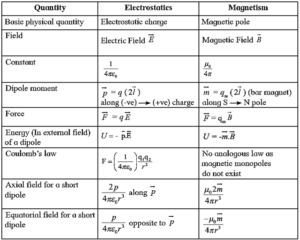
Equivalent physical quantities in electrostatics and magnetism :
Expression for the magnetic induction at (i) an axial point (ii) an equatorial point due to a short magnetic dipole :
The magnetic induction (B) at a point due to a short magnetic dipole of magnetic moment m is given by
B = \((\frac{μ_0}{4π}.\frac{m}{r^3})\sqrt{3cos^2θ+1}\)
where r is the distance of the point from the centre of the dipole, along a line making an angle θ with the dipole axis.
If \(vec{B}\) makes an angle ∝ with this line, tan ∝ = \(\frac{1}{2}tan\,θ\)
For a point at distance r along the axis of the dipole, θ = 0° or 180°. ∴ cos θ = ±1.
∴ Baxis = \(\frac{μ_0}{4π}.\frac{2m}{r^3}\)
For a point at the same distance r along the equator of the dipole, θ = 90 ° or 270 °.
∴ cos θ = 0
∴ Beq = \(\frac{μ_0}{4π}.\frac{m}{r^3}\)
∴ Baxis = 2Beq
- For θ = 0°, tan θ = 0 and ∝ = 0°;
- For θ = 180°, tan θ = 0 and ∝ = — 180°.
In both cases, \(\vec{B}_{axis}\) is along \(\vec{m}\).
- For θ = 90°, tan θ = ∞ and ∝ = 90°;
- For θ = 270°, tan θ = ∞ and ∝ = 270°.
In both cases, \(\vec{B}_{eq}\), is opposite to \(\vec{m}\).
Gauss' Law of Magnetism :
Equivalence between a magnetic dipole and a current-carrying solenoid :
Solenoid : A solenoid is a long wire wound in the form of a helix. An ideal solenoid is tightly wound and infinitely long, i.e., its turns are closely spaced and the solenoid is very long compared to its cross—sectional radius.
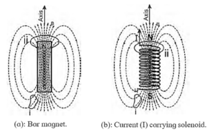
- Each turn of a current-carrying solenoid acts approximately as a circular current loop and the net magnetic induction is the vector sum of the inductions due to all the turns.
- In the case of a tightly-wound solenoid of finite length (see Fig.), the magnetic field lines are approximately parallel only near the centre of the solenoid, indicating a nearly uniform magnetic induction there.
- However, close to the ends, the field lines diverge from one end and converge at the other end. This field distribution is similar to that of a bar magnet.
- Thus, one end of the solenoid behaves like the north pole of a magnet and the other end behaves like the south pole. The field outside is very weak near the midpoint.
- The magnetic field of a current carrying solenoid is similar to that of a bar magnet.
Gauss’ law in magnetism : The net magnetic flux Φm through a closed surface of arbitrary shape is zero.
In integral form, Φm = \(\oint \limits_{s} \vec{B}.\vec{dS}\) = 0
where the integration is over a closed surface S.
Explanation : Below figure schematically shows the magnetic field lines of a bar magnet and a current—carrying solenoid, and the electric field lines of an electric dipole. The dotted curves S1 and S2 represent Gaussian surfaces.
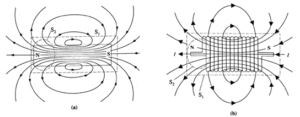
In Figs. (a) and (b), the number of magnetic field lines entering each of the surfaces S1 and S2 are equal to the number of lines leaving the respective surfaces. That is, the net flux Φm through them is zero. Although S2 appears to enclose the north pole, Φm = 0 means that there is no magnetic charge there.
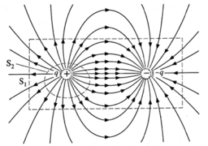
For an electrostatic case, however, Gauss’ law states that the net electric flux through a closed surface S is Φe = \(\oint \limits_{s} \vec{E}.\vec{dS}=\frac{∑q}{ε_0}\), where ∑q is the net electric charge enclosed by S.
In below Fig. Φe =0 through S1 and ∑q is also zero, while there is a net outward flux through S2 and ∑q = + q, both cases consistent with Gauss’ law and the fact that an isolated electric charge exists.
Thus, by Gauss’ law in magnetism,
- magnetic monopoles do not exist — magnetic field is dipolar in character.
- net magnetic flux through any volume is always zero.
If magnetic monopoles exist : Gauss‘ law in magnetism would be analogous to that in electrostatics : The net magnetic flux through a surface enclosing a monopole of pole strength qm would be equal to the product μ0 qm, where μ0 is the permeability of free space.
\(\oint \limits_{s} \vec{B}.\vec{dS}\) = μ0 qm
where the integration is over the closed surface S enclosing the magnetic monopole.
Earth’s Magnetism :
Geo Magnetism :
- If a bar magnet or a magnetic needle suspended freely in air always aligns itself along geographic N-S direction. If it has a freedom to rotate about horizontal axis, it inclines with some angle with the horizontal in the vertical N-S plane.
- It indicates that there is some magnetic field present everywhere on the Earth. This is called Terrestrial Magnetism. It is extremely useful during navigation.
Magnetic parameters of the Earth are described below :
- The magnetic lines of force enter the Earth's surface at the north pole and emerge from the south pole.
- Unless and otherwise stated, the directions mentioned (South, North, etc.) are always, Geographic.
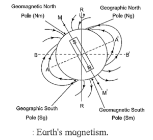
Geographic axis : The imaginary line through the centre of the Earth about which the Earth spins is called the geographic axis.
- Its northern end on the Earth’s surface is called the North Pole or the 90° N latitude. Its southern end is called the South Pole or the 90° S latitude
Geographic meridian : The vertical plane at a place through the geographic North and South Poles (i.e., containing the geographic axis) is called the geographic meridian at that place.
Geographic equator :The great circle (0° latitude) on the Earth’s surface, in a plane perpendicular to the geographic axis and passing through the Earth's centre, is called the geographic equator.
Magnetic axis : The axis of the dipolar geomagnetic field is called the magnetic axis of the Earth or the geomagnetic axis. Its northern and southern ends on the Earth's surface are called the north magnetic pole and south magnetic pole, respectively. It is inclined at 11.3° to the geographic axis.
Magnetic meridian : The vertical plane at a place passing through the north and south magnetic pole and containing the magnetic axis (i.e., containing the direction in which a compass needle sets itself at that place) is called the magnetic meridian at that place.
Magnetic equator: The great circle on the Earth’s surface in a plane perpendicular to the geomagnetic axis is called the magnetic equator. On the magnetic axis, the dip is zero.
- In India, the magnetic equator passes through the town Kollam near Thiruvananthapuram.
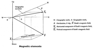
Magnetic elements at a place :
The magnitude and direction of the magnetic field of the Earth at a place on the Earth's surface are completely specified by the declination, dip and horizontal component of the field at that place. These are known as the magnetic elements at that place.
(i) Declination : The direction in which a compass needle points at a particular place makes an angle with the geographical meridian. The vertical plane containing the direction in which a compass needle sets itself at a place is called the magnetic meridian at that place. The angle between the magnetic and geographic meridians is called the declination.
- Magnetic declination does not depend latitude. The lines of flux are pretty random.
(ii) Dip (or inclination) : At a place on the Earth's surface, the magnetic induction of the Earth \(\vec{B}\) is, in general, inclined to the surface. A dip needle placed with its plane in the magnetic meridian points in the direction of \(\vec{B}\) at that place. The angle which a dip needle makes with the horizontal is the angle between \(\vec{B}\) and the horizontal. This angle is called the dip or inclination, δ at the place.
- On the magnetic equator, dip angle = 0°. At the north and south magnetic poles, the dip angle is 90° and 270° degrees.
(iii) Horizontal component of the Earth's magnetic induction: At a place on the Earth's surface the horizontal component of the Earth's magnetic induction is
BH = B cos δ
where δ is the dip and B is the magnitude of the Earth's magnetic induction at that place.
The vertical component of the Earth's magnetic induction at the place is
BV = B sin δ
Then, tan δ = BV/BH and B = \(\sqrt{B_v^2+B_H^2}\)
Special cases
- At the magnetic North pole, \(\vec{B}=\vec{B_V}\) directed upward, BH = 0 and Φ = 900.
- At the magnetic south pole, \(\vec{B}=\vec{B_V}\)directed upward, BH = 0 and Φ = 2700
- Anywhere on the magnetic great circle (magnetic equator) B = BH along South to North, BV= 0 and Φ = 0
Magnetic maps of the Earth:-
Magnetic maps : Magnetic elements of the Earth (BH, α and Φ) vary from place to place and also with time. The maps providing these values at different locations are called magnetic maps.
Uses :
- These are extremely useful for navigation.
- Local variation in Earth‘s magnetic field, called magnetic anomalies, result from variations in the chemistry or magnetism of the rocks.
- Magnetic surveys (i.e., maps of variation) over an area are valuable in detecting buried structures and archaeological artefacts.
Isomagnetic charts : Magnetic maps drawn by joining places with the same value of a particular element are called Isomagnetic charts.
- Lines joining the places of equal horizontal components (BH) are known as ‘Isodynamic lines’
- Lines joining the places of equal declination (α) are called Isogonic lines.
- Lines joining the places of equal inclination or dip (Φ) are called Aclinic lines.
Types of isomagnetic charts :
- Isodynamic chart—it can be of three types showing either total field B, horizontal component of the field BH or vertical component of the field BV.
- Isogonic chart
- Isoclinal or isoclinic chart.
We reply to valid query.